EDGAP (Exponentially Decayed Geometric Average Price)

EDGAP is an exponential moving average for geometric pricing in a CPAMM (Constant Product Automated Market Maker). It tracks the decaying averages of “token0 per liquidity” and “token1 per liquidity,” continuously weighing recent data more than older data to reflect current market conditions.

Why Use EDGAP?

• Smooth Price Updates
  It reduces short-term volatility by blending old and new data over time, so sudden price changes get dampened.

• Exponential Decay
  The influence of older data decays exponentially with a configurable half-life: each half-life period effectively reduces the weight of old data by 50%.

• Geometric Focus
  By tracking token0-per-liquidity and token1-per-liquidity, you can compute a stable geometric mean price for the pool, especially suited for constant-product AMMs.

Key Concepts

1. Half-Life (Seconds)
   Represents how quickly old data “decays.” After each half-life period:

   • The influence of old data is halved.
   • The most recent data gets proportionally more weight.

2. Token0 / Token1 per Liquidity

   • Instead of tracking absolute token amounts, EDGAP tracks normalized values (tokenXPerLiquidity) to maintain consistent comparisons across changing liquidity conditions.

3. Exponential Moving Average Calculation

• alpha = HalfLife.calculateHalfLifeValue(halfLifeSeconds, 1e18, timeElapsed)
• newAverage = (oldAverage * alpha) + (latestData * (1 - alpha))

4. Decay Logic

   • Older data fades out exponentially.
   • New data is integrated smoothly, preventing sharp, abrupt shifts in price.

5. Geometric Average Price
   Once the EDGAP values for token0 and token1 are known, you can compute a price like:

   price = token1PerLiquidity / token0PerLiquidity

   under an exponential weighting scheme that updates every time a pool event occurs (swap, add/remove liquidity, etc.).

Quick Usage Overview

1. Initialize

   • On the first pool update, store token0PerLiquidity and token1PerLiquidity in your EDGAP struct.

2. Update

   • Each time new data arrives (e.g., new amounts after a swap), call updateEDGAP() with the current halfLifeSeconds.
   • The library internally decays the old values and mixes in the new values.

3. Query

   • Use functions like getPriceOnePerZeroWAD or getRatioZeroPerOne64x64 to retrieve the current exponentially decayed price.

EDGAP Visualizer

Below is a simplified conceptual diagram of how EDGAP updates over time, illustrating the effect of exponential decay on a price metric:

 Time (seconds) --->

 ┌────────┐
 │ Old    │     - Past data from previous blocks
 │ Data   │
 └────────┘
      | (decayed by α)
      v
┌─────────────────┐
│ Weighted Average │    EDGAP blends old data with new data:
├─────────────────┤    weightedAverage = oldAverage*α + newData*(1-α)
│   α => decays   │
└─────────────────┘
      | (combine)
      v
┌────────┐
│ New    │     - Current block's updated
│ Data   │       token0/token1 per liquidity
└────────┘

1. Old Data: Represents previously stored EDGAP values.
2. New Data: The fresh measurements of token0PerLiquidity and token1PerLiquidity.
3. α (Alpha): A weight factor derived from the configured half-life and the time elapsed.
4. Exponential Decay: The older EDGAP values are scaled by α, so they decay exponentially as time passes.

This visual helps you see how EDGAP seamlessly transitions from old data to new, preserving historical context while staying responsive to the latest changes.

EDGAP in Action: Step-by-Step Charts

Below is a simplified illustration of how EDGAP (Exponentially Decayed Geometric Average Price) updates as new data points arrive. These examples assume we’re tracking a single EDGAP value, but the same logic applies to both token0PerLiquidity and token1PerLiquidity in parallel.

In this example, the half life period of the EDGAP is 1 day.

Chart 1: First Data Point

In an EDGAP setup, the first data point is simply recorded. EDGAPs need at least two data points to be computed.

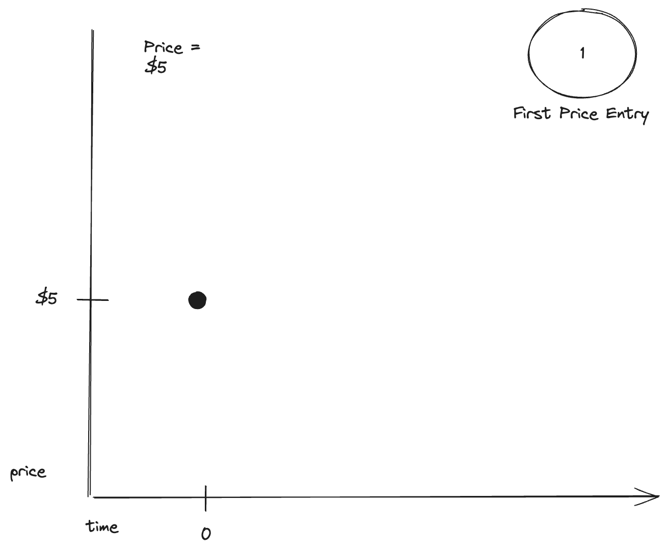
Chart 2: Second Data Point

• 1 day has passed
• A new data price entry comes in at $10

In an EDGAP setup, the second data point is also simply recorded.

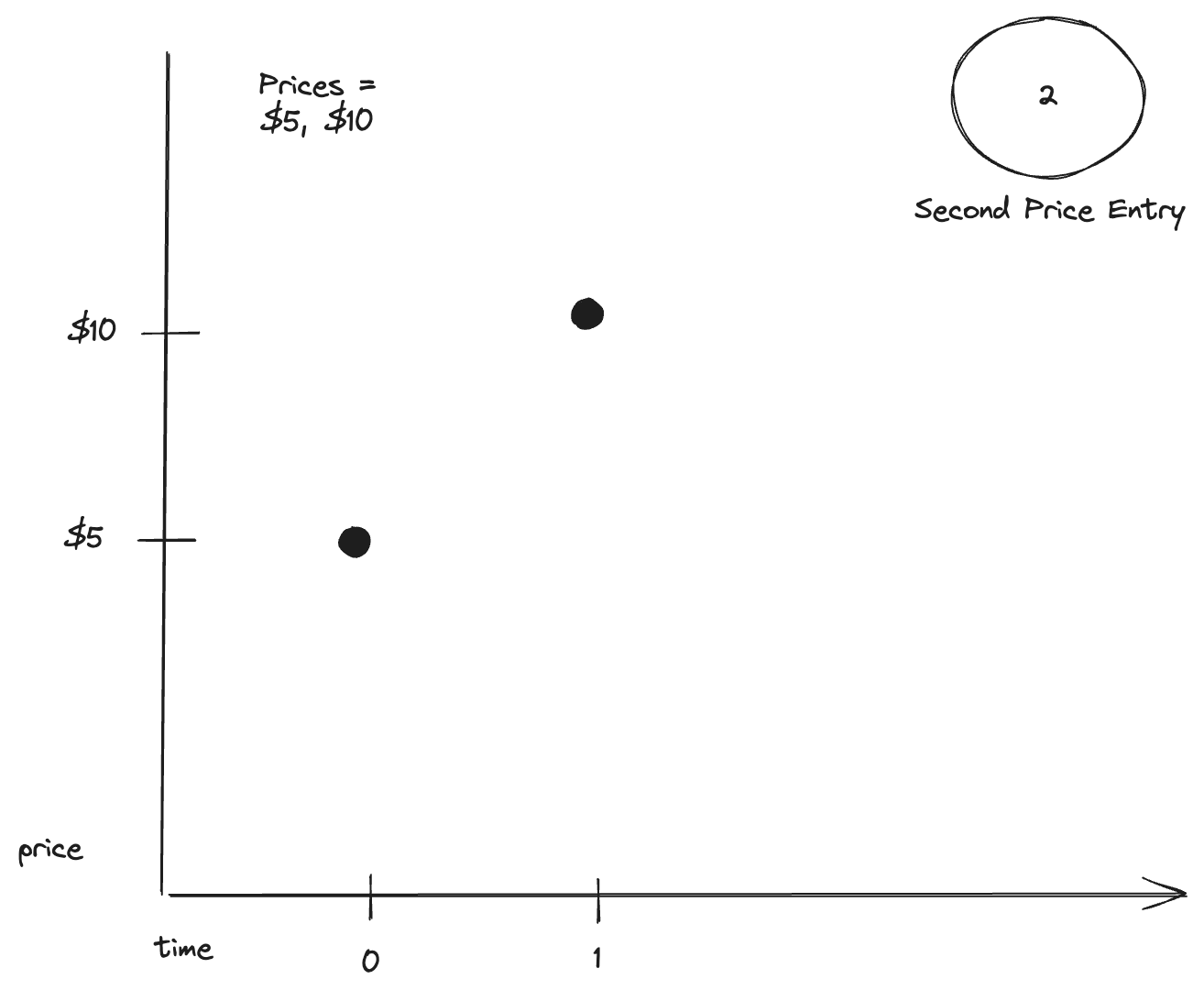
Chart 3: Two data points, one day passed

Now that there are two data points, an EDGAP can be computed. An EDGAP is computed by:

EDGAP Price = firstPrice * 0.5^(t/T) + secondPrice * (1 - 0.5^(t/T))

Assume one day has passed, the EDGAP can be computed as:

$5 * 0.5^(1) * $10 * 0.5^(1) = $7.5

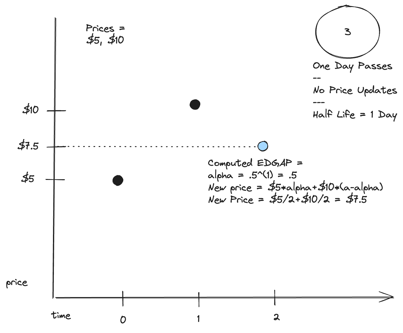
Chart 4: One more day passes, new price update

Assume one more day has passed (for a total of 2 days since our last price entry). A new price entry comes in at $2.

The EDGAP will store the most recently computed price as well as the new price entry.

Because two days have passed since the latest price entry, the EDGAP price becomes

$5 * 0.5^(2) * $10 * (1 - 0.5^(2)) = $8.75.

The EDGAP becomes the older price and the new price ($2) becomes the newer price that we will use to compute the EDGAP at the next price entry.

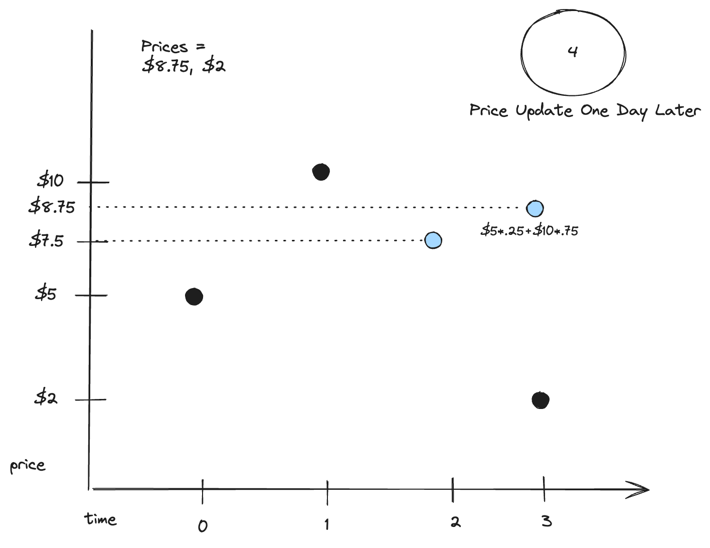
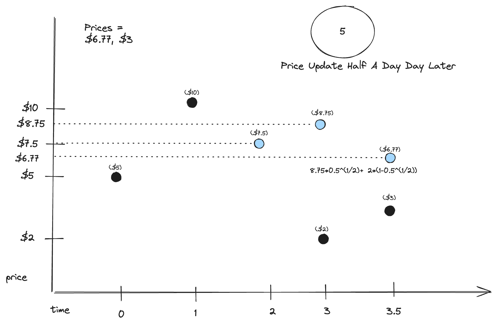
Chart 5: Half a day passes, new price update

Assume half a day passes since the last update and there is a new price update of $3.

The new computed EDGAP becomes

$8.75 * 0.5^(0.5) + $2 * (1 - 0.5^(0.5)) = $6.77

The EDGAP will store the most recently computed price as well as the new price entry.

This process continues to happen for each new price update.

Key Points

• EDGAP is an exponentially decaying moving average of the price of a token in a CPAMM
• EDGAP relies on having two geometric means (price) and blending them together based on the half life period.
  • To combine two prices, the formula is:

EDGAP Price = price1 * 0.5^(t/T) + price2 * (1 - 0.5^(t/T))